Identifying My Regular Commute Routes To Work

For the last 18 months the Walmer Street Bridge has been closed (until recently). While it was closed, the detour added about 10 minutes to my commute. This closure and subsequent detour led me to reflect on the various distinct routes I’ve taken to work over the years, and what sets each one apart.

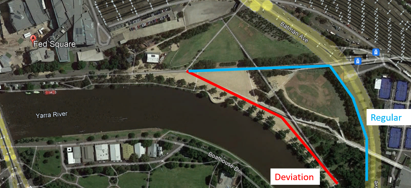
For instance, consider a morning when I take a slightly different path from my usual route, a variation I refer to as the ‘Deviation’ (see image below). Does this minor deviation qualify as an entirely new way of commuting to work? What if I briefly rode on the wrong side of the road for just 10 meters. While technically this is a different route, practically it’s not significantly distinct from my usual route.

Example Deviation — A deviation (red) from typical route to work (blue). The deviation is a shortcut along a sandy section of the Yarra River trail.

Before we can determine whether a route deviation constitutes an entirely different route, we need the ability to objectively differentiate between routes, preferably in a programmable way.

The following examples show how this can be achieved.

Example 1: My lunchtime walk to Safeway Woolworths

Typically, my route involves initially heading west on Collins Street and then turning north onto Merchant Street.

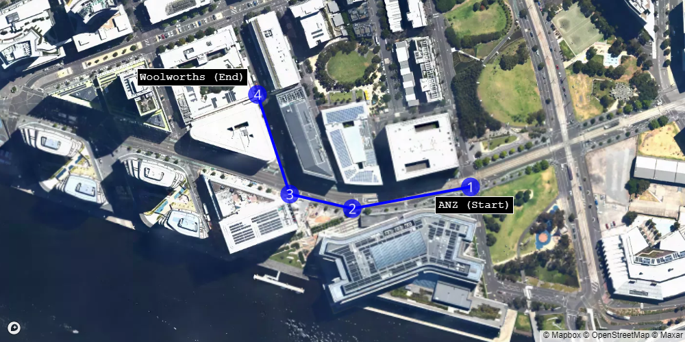
Typical walk to Woolworths — My typical lunchtime walking route from my office to Woolworths.

Sometimes, though very rarely, I would walk west on Collins St, turn right onto Import Lane, and then take a left along a pedestrian alley.

Rare route to Woolworths — My less-travelled walking route from the office to Woolworths, overlaid in red as the 'Alternative Route', with the regular route shown in blue.

These two routes can be represented as sequences of four pairs of latitude and longitude coordinates.

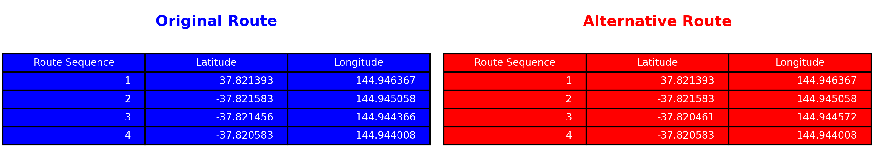
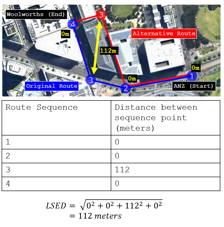
Both routes shown as four pairs of latitude and longitude coordinates. — Original and Alternative routes being represented as a sequence of four latitude-longitude pairs.

To determine whether two routes are identical, or to quantify their differences if they are not, we can use the Lock-step Euclidean Distance (LSED)*. To visualise the calculation of this distance, we first compute the ‘as-the-bird-flies’ distance between corresponding points on each route. These distances are then squared, summed, and finally, the square root is taken.

In the route below, the LSED is calculated to be 112 meters. As expected, the LSED is non-zero, primarily because sequence point 3 is located at different positions in each route, while all other sequence points are identical.

This all seems pretty straightforward; however, what happens when one route has more sequence points than the other?

*Note that technically this is not the Euclidean distance but the “geodesic distance” which measures the distance between two points on the Earth’s surface. The basic idea still applies.

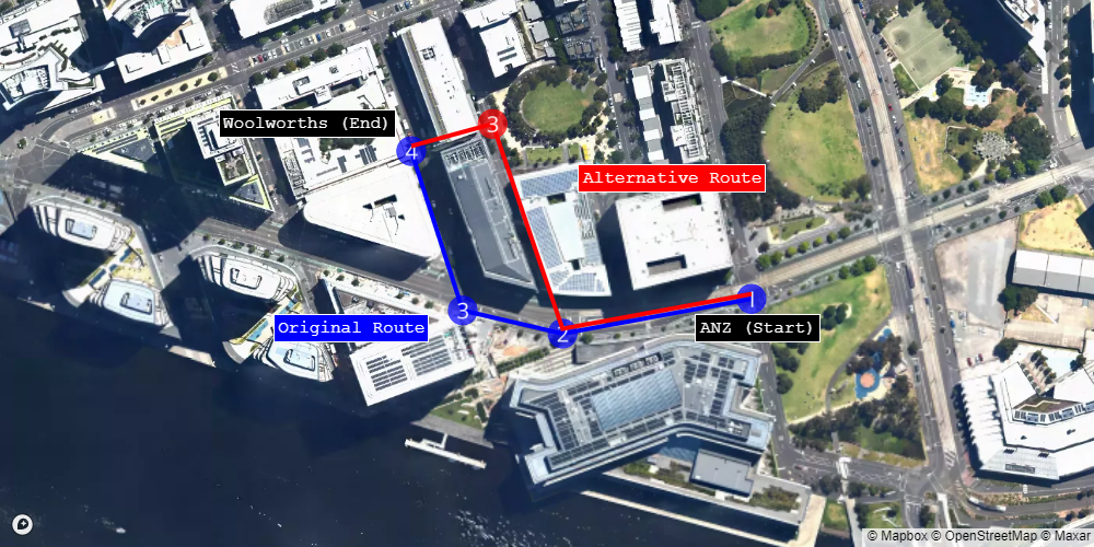
Example 2: My complicated lunchtime walk to Woolworths

In this example, the alternative route involves first heading north and weaving through the buildings, totalling six route sequence points.

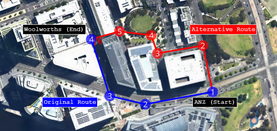
The complicated alternative route requires six sequence points.

If we attempt to calculate the LSED as we did in Example 1, we naturally start by comparing corresponding points:

Point 1 of the original route to point 1 of the alternative route
Point 2 of the original to point 2 of the alternative
Point 3 of the original to point 3 of the alternative
Point 4 of the original to point 4 of the alternative

However, what happens when there is no corresponding point 5 in the original route to compare with point 5 of the alternative route? The same issue arises for point 6 of the alternative route.

As the name suggests, the Lock-step Euclidean Distance breaks down because the points are no longer in ‘lock-step’.

Introducing Dynamic Time Warping (DTW)

In Example 2, we identified a limitation of the Lock-step Euclidean Distance approach in that it is unable to effectively handle cases where one route has a different number of points compared to another.

As an alternative, the Dynamic Time Warping (DTW) algorithm can be employed, which calculates the (minimum) cost of aligning two routes, even if they vary in number of route points. In this case, the cost of aligning the two routes becomes our method of measuring how similar or dissimilar two routes are.

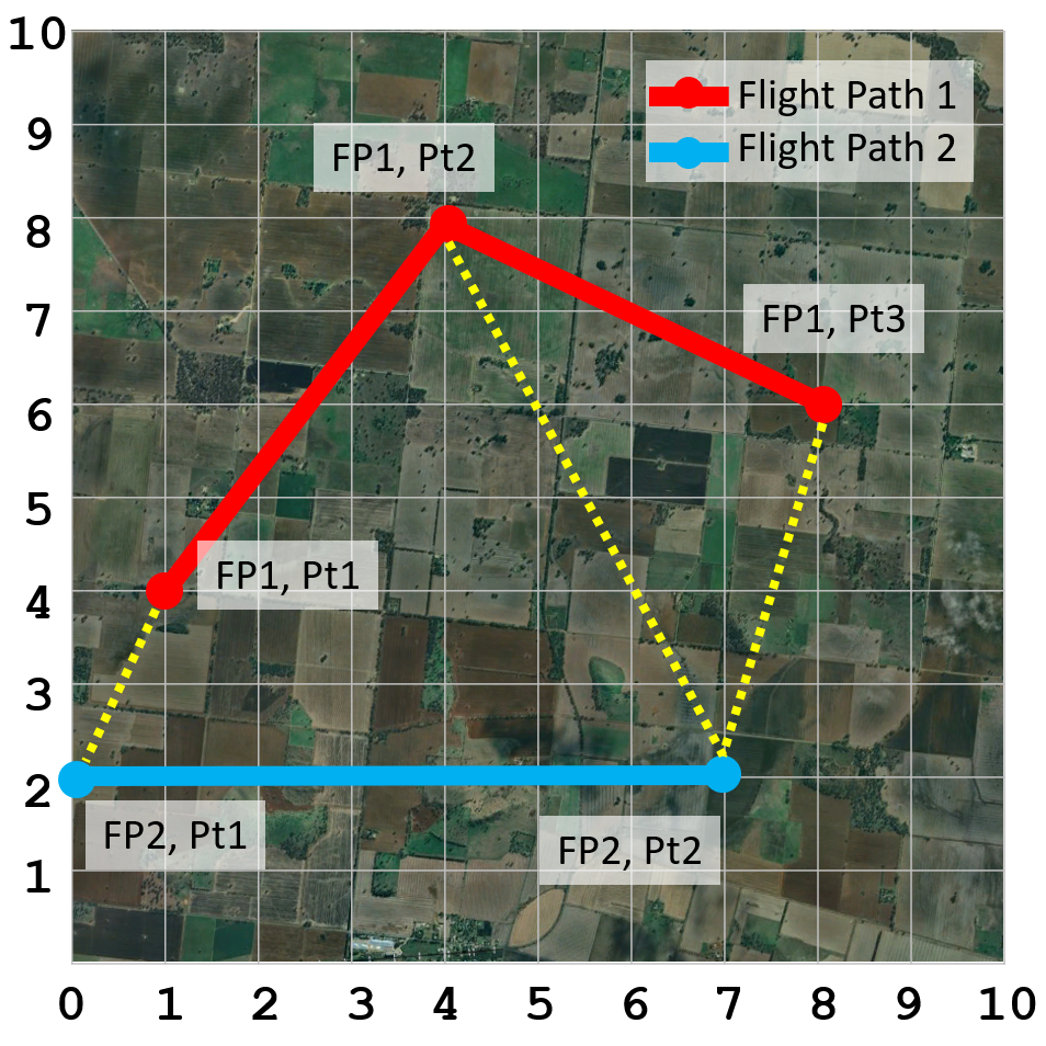
To demonstrate how the DTW algorithm works, let’s consider a simple application: comparing the flight paths of two birds in the sky. To simplify further, we will assume that the coordinate space is an x-y plane and the birds maintain the same altitude during their flight. Bird 1 follows flight path 1, while bird 2 follows flight path 2.

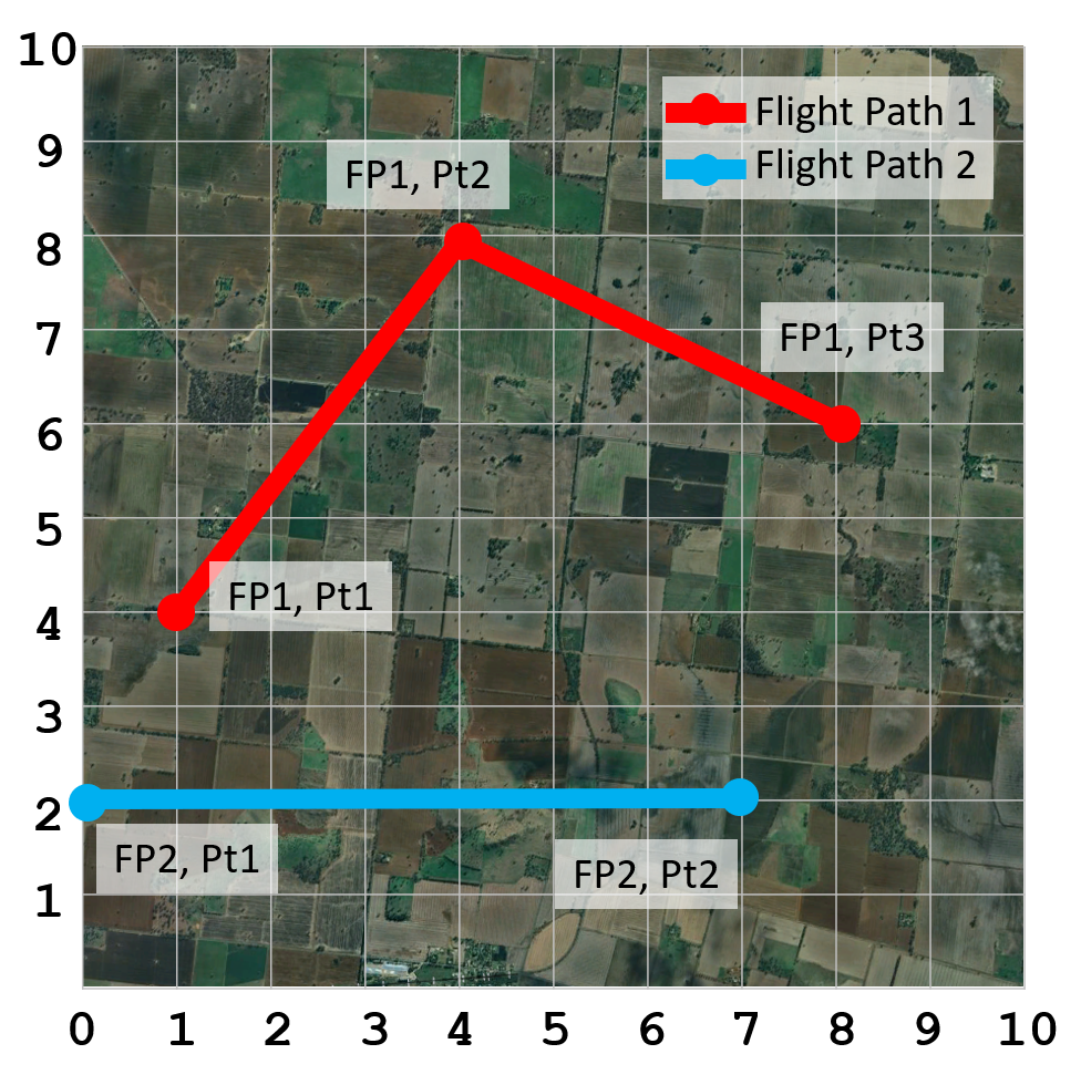
The flight paths of two birds (bird 1 and bird 2) travelling at the same altitude. "Point" = "Pt" for brevity.

The first step of the algorithm is to construct a matrix of all possible squared distances between each point on the birds’ flight paths. Then, starting at the bottom-left corner of the matrix, we move towards the top-right corner while minimising the sum of the squared distances (i.e., the values in each cell of the matrix). The path, highlighted in the yellow matrix cells, represents the pairs of points from each respective bird’s flight path that are to be aligned. The cost of aligning these points corresponds to how similar the two flight paths are.

There are a few additional rules to the DTW algorithm which are covered here.

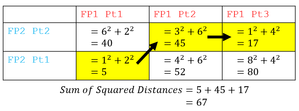
A matrix containing squared distances between each point on the birds' flight path.

We can also visualise which points are aligned by the DTW algorithm by drawing a dashed yellow line between them. It’s worth noting at this point that there are other possible ways of aligning the two birds’ flight paths. However, we need a consistent approach to aligning the paths — that is, minimising the squared distances — so that we can consistently compare any pair of flight paths.

Points aligned by the DTW algorithm have a dashed yellow line drawn between them.

Now that we have a good understanding of the DTW algorithm and its ability to programmatically determine the similarity between two flight paths (or routes), let’s apply it to actual route data that I’ve captured using Strava while riding my bike to work.

Preparing Bike Route Data

Strava makes it very easy to bulk download your entire activity history.

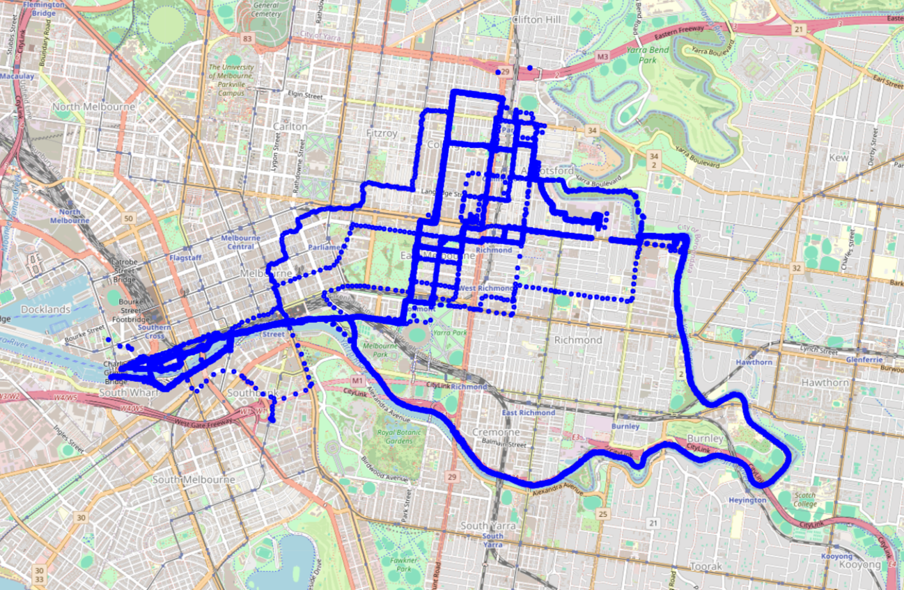
Since I’ve been using Strava from around 2010, I have numerous bike ride activities that neither start at my current home nor end at my current workplace. To optimise the DTW algorithm’s ability to assess route similarity, I will include only those routes in the dataset that start within a 200 meter radius of my home and end within a 200 meter radius of my workplace. Applying this filter leaves us with data corresponding to around 200 rides to work.

To improve the accuracy of the DTW algorithm and ensure privacy in this blog post, I will also remove data points from the routes that are within a 200 meter radius of both my home, workplace and gym, where GPS signals tend to be less reliable.

Upon visually inspecting these routes displayed on a map, we can identify some common routes that I frequently take, indicated by thicker and less patchy blue lines.

Testing the DTW Algorithm

Now that we have 200 historical routes ready for analysis, we can begin applying the DTW algorithm. I also want to acknowledge a helpful write-up and sample code that made it easier to put this algorithm into practice.

Before we run DTW across all the data, let’s test how it performs on two similar but slightly different routes to work.

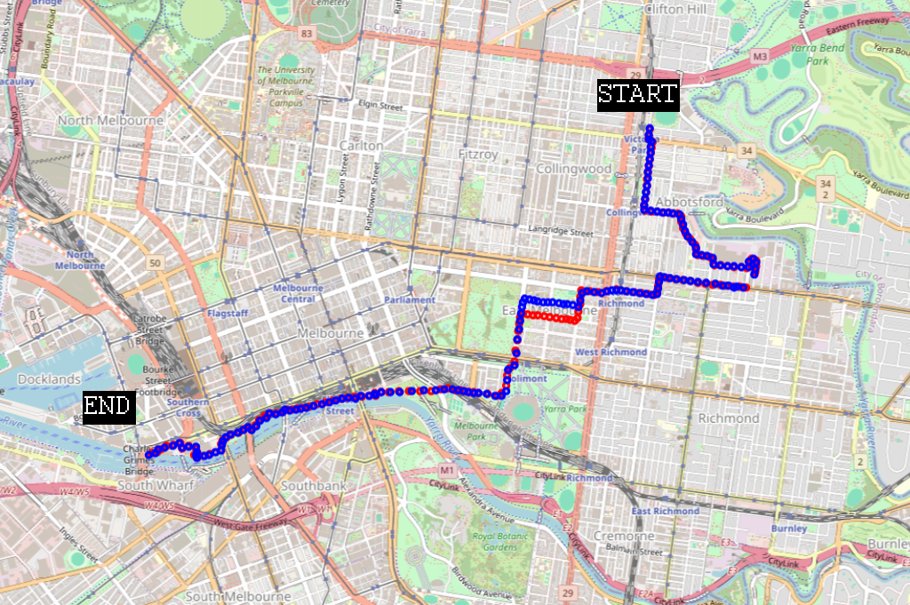
A map showing two similar routes from home to work.

Given that the DTW algorithm’s objective is to align all points with minimal cost, we can visually represent this with a matrix containing the distances between all points along both routes. In the matrix below, there are too many distance values to show (155 x 158 matrix cells) so a colour gradient has been used instead. Dark areas represent a large distance between two points from different routes and lighter areas indicate short distances between points from different routes. The optimal way to align both routes to one-another can be achieved with the alignment shown by the green line.

We can also see that the two routes generally track each other well except for a period where the blue route is the first to turn west off a street. This deviation can also be seen in the distance matrix.

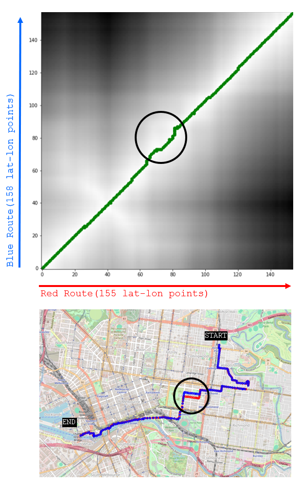
A deviation between two routes represented as a distance matrix between all points of both routes. Circled are deviations from almost-perfect alignment of the two routes.

In this example, the total distance required to align all points is 4.44km. In other words, the similarity between the two routes is represented by a distance of 4.44km. I was expecting a smaller number; however, given that most points are not in phase, the distance needed to align the points is often non-zero. In the next section, we’ll see that 4.44km is actually a relatively small distance for aligning all points between two routes.

The DTW distance (km) between the first 10 points of both routes shown above. Small phase shifts and GPS inaccuracy results in non-zero distances.

DTW Results and Clustering ‘Distinct’ Routes

In total, approximately 200 routes were analysed for similarity, leading to the calculation of DTW (Dynamic Time Warping) distances for about 19,900* unique pairs of routes.

*200ⁿC₂ = 200! / (2! × (200-2)!)

To cluster the routes, I adopted a straightforward method that was perhaps less than ideal but still provided some good insights. The process for clustering was as follows:

Select a route and find other routes with a DTW distance of less than 10km. Group these routes into ‘cluster 1’.
Move to the next route and repeat the process, ensuring to exclude any routes already included in ‘cluster 1’.
Continue with this approach, forming new clusters as necessary.

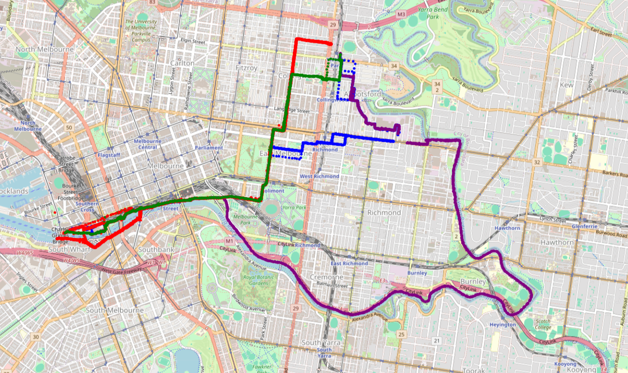
By colour-coding each cluster of routes on the map, we can clearly see that the crude clustering approach has produced reasonably effective results. As I personally participated in creating the data for these routes, I’m able to provide my own narratives for each one.

Specifically:

Red = This is a direct route, where I cross Hoddle Street first
Green = This is an alternative direct route, where I cross Johnston Street first
Blue = This route involves riding to the gym then continue to work
Purple = This is a longer route for cardio exercise, taking a detour along the Yarra Trail.

Unfortunately, the Walmer Street Bridge detour is not represented as an additional cluster because the Strava ride data for these routes was captured in a format that caused challenges for processing with the DTW algorithm.